Algorithms
No raw loops.
Programming is about computing something. Algorithms are an abstraction of computation, and every program is an algorithm. It is easy to be distracted by class hierarchies, software architecture, design patterns, etc. Such things are helpful only insofar as they aid in implementing a correct and efficient algorithm.
Algorithm (n.): a process or set of rules to be followed in calculations or other problem-solving operations, especially by a computer (New Oxford American Dictionary).
When designing a program, we start with a statement of what the program will do, and we refine that statement until we reach a level of detail sufficient to begin the implementation. The process is iterative as we discover details that inform and change the overall design.
For each component of the design, we will have a statement of what the component is or does. Components that do something are operations, and the statement of what they do form the basis for the operations contract.
Consider a simple example. Suppose we are building a drawing tool and want to remove a selected shape from an array. The naive implementation is a loop that scans for the shape and erases it.
 struct Shape { var isSelected: Bool }
/// Removes the selected shape.
func removeSelected(shapes: inout [Shape]) {
    for i in 0..<shapes.count {
        if shapes[i].isSelected {
            shapes.remove(at: i)
            break
        }
    }
}
We can extend the requirement to allow the user to select multiple shapes and modify the code to remove the selected shapes. The loop becomes more complicated. Removing one element shifts the indices of the remaining ones, so the code must handle an additional case.
 struct Shape { var isSelected: Bool }
/// Remove all selected shapes.
func removeAllSelected(shapes: inout [Shape]) {
    var i = 0
    while i < shapes.count {
        if shapes[i].isSelected {
            shapes.remove(at: i)
            // Don't increment i; the next element is now at position i
        } else {
            i += 1
        }
    }
}
We could simplify the loop by reversing the direction of iteration, since only subsequent indices are affected by the removal this removes the fix-up.
 struct Shape { var isSelected: Bool }
/// Remove all selected shapes.
func removeAllSelected(shapes: inout [Shape]) {
    for i in (0..<shapes.count).reversed() {
        if shapes[i].isSelected {
            shapes.remove(at: i)
        }
    }
}
The code is simpler, but it has a significant flaw. For each selected item we perform a remove which is linear with the number of subsequent elements. The performance is then O(n^2).
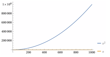
At scale, quadratic behavior will make our application unusable.
Intent to Mechanism
We can remove the selected shapes more efficiently. The trick is to collect all of the unselected shapes at the start of the array, and then remove the remaining shapes all at once. We don’t care about the shapes to be removed or their order.
To design an algorithm to collect the unselected shapes, we use a common technique of stating the postcondition and then seeing if there is a way to extend the postcondition to additional elements.
The desired postcondition for collecting the unselected shapes is that all the
unselected shapes are in the range 0..<p in their original order, where p is
the count of unselected shapes.
Now, consider if this condition holds up to some point, r, instead of to the
end of the array, where r... are the remaining shapes that may or may not be
selected. To advance r we examine the shape at shapes[r], if it is not
selected, we need to add it to 0..<p.
There are two ways1 we could do that. The first is to copy the shape shapes[p] = shapes[r], but there are costs to copying . The other option is to swap the element at
shapes[r] with the element at shapes[p].
Both approaches will preserve the relative order of the unselected shapes. Now we can write the code:
 struct Shape { var isSelected: Bool }
/// Remove all selected shapes.
func removeAllSelected(shapes: inout [Shape]) {
    var p = 0

    for r in 0..<shapes.count {
        if !shapes[r].isSelected {
            shapes.swapAt(p, r)
            p += 1
        }
    }

    // Remove all selected shapes from the end
    shapes.removeSubrange(p...)
}
Take a moment to prove to yourself that the loop is correct.
The act of verifying a loop requires us to establish:
- A loop invariant that holds before each iteration (including the first), and at loop termination.
- A variant function a notional function that maps to a strictly decreasing value on each iteration to prove termination
- A postcondition that is a statement of the loop invariant at loop termination.
Our loop invariant is almost completely covered by the description of our algorithm:
- Loop invariant:
0..<pcontains all unselected shapes in0..<r.p..<rcontains all selected shapes in0..<r- for all
iin0..<p, theith unselected element of the original array is in positioni(i.e., unselected shapes are in their original order).
- Variant function:
- The difference between
shape.countandris reduced by one at each iteration. The loop exits when the difference is zero.
- The difference between
- Postcondition:
- When the loop exists,
r == shapes.count, all unselected elements appear in0..<pin their original order and all the selected elements are inp...
- When the loop exists,
As an exercise, look back at the two prior implementations of
removeAllSelected() and prove to yourself that the loops are correct.
As with contracts, the processes of proving to ourselves that loops are correct is something we do informally (hopefully) every time we write a loop. Our code reviewers should also verify the loop is correct. Even in this simple example it is easy to make a small mistake that could have serious consequences.
The best way to avoid complexity of loops is to learn to identify and compose algorithms. The loop we just implemented is a permutation operation that partitions our shapes into unselected and selected subsequences. The relative order of the shapes in the unselected sequence is unchanged. This property is known as stability, so this operation is a half-stable partition. The algorithm is not specific to shapes so we can lift it out into a generic algorithm.
extension MutableCollection {
    /// Reorders the elements of the collection such that all the elements that match
    /// the given predicate are after all the elements that don’t match, preserving
    /// the order of the unmatched elements. Returning the index of the first
    /// element that satisfies the predicate.
    mutating func halfStablePartition(
        by belongsInSecondPartition: (Element) -> Bool
    ) -> Index {
        var p = startIndex

        for r in indices {
            if !belongsInSecondPartition(self[r]) {
                swapAt(p, r)
                formIndex(after: &p)
            }
        }

        return p
    }
}
Given halfStablePartition() we can rewrite removeAllSelected().
 struct Shape { var isSelected: Bool }
 extension MutableCollection {
   /// See the full `halfStablePartition` implementation earlier in this chapter.
   mutating func halfStablePartition(
     by belongsInSecondPartition: (Element) -> Bool
   ) -> Index {
     fatalError()
   }
 }
func removeAllSelected(shapes: inout [Shape]) {
    shapes.removeSubrange(shapes.halfStablePartition(by: { $0.isSelected })...)
}
Although we can’t do better than linear time, our implementation of
halfStablePartition() is doing unnecessary work by calling swap when p == r.
As an exercise, before entering the loop, find the first point where a swap will
be required, prove the new implementation is correct. Create a benchmark to
compare the performance of the two implementations.
Often, we view efficiency as the upper-bound (big-O) of how an algorithm scales in the worst case. Scaling is important, but so are metrics like how much wall clock time the operation takes or how much memory the operation consumes. In the software industry if a competitors approach takes half the time or runs in production at half the energy costs, that could be a significant advantage.
We define efficiency of an operation as the minimization of resource the operation uses to calculate a result. The resources include:
- time
- memory
- energy
- computational hardware
Because memory access is slow, energy consumption is largely determined by the amount of time an operation takes, and computational hardware is often underutilized, we prioritize optimizing time. But as we will see in the Concurrency chapter, balancing all of these resources is critical for an efficient system design.
When designing algorithms it is important to have a rough sense of the cost of primitive operations to guide the design. Some approximate numbers by order of magnitude2:
| Cycles | Operations |
|---|---|
| 10^0 | basic register operation (add, mul, or), memory write, predicted branch, L1 read |
| 10^1 | L2 and L3 cache read, branch misprediction, division, atomic operations, function call |
| 10^2 | main memory read |
| 10^3 | Kernel call, thread context switch (direct costs), exception thrown and caught |
| 10^4 | Thread context switch (including cache invalidation) |
A rotation expresses “move this range here.” A stable partition expresses “collect the elements that satisfy this predicate.” A slide is a composition of rotations. A gather is a composition of stable partitions.
The loops are still there. They are no longer our problem.
Real programs rarely need a single loop. They need several: one loop to find something, another to remove it, another to insert it somewhere else, and perhaps another to repair the structure afterward.
Each loop is simple in isolation. Together they form a fragile tangle of index adjustments, off‑by‑one corrections, and implicit assumptions about the state of the data.
A loop is a mechanism. It tells the computer how to step, but it does not tell the reader what is being computed.
The problem is not the loops themselves. The problem is that they are exposed. They are raw. They are unencapsulated.
Encapsulation is the difference between a loop and an algorithm. A loop is a mechanism. An algorithm is a named, reusable composition that hides the mechanism and exposes the intent.
A raw loop is a loop that appears directly in application code. It exposes mechanics instead of intent. It forces the reader to reason about control flow instead of the operation being performed. Raw loops are unencapsulated loops.
When I say “no raw loops,” I do not mean “no loops.” Every algorithm contains loops. The problem is not iteration; the problem is exposure. A raw loop is a loop that appears in application code, unencapsulated, forcing the reader to reason about mechanics instead of intent. Real operations often require several loops—one to find something, another to remove it, another to insert it somewhere else. Left raw, these loops accumulate into brittle, low-level code. Encapsulated as algorithms, they become simple, composable building blocks.
We do not avoid loops. We avoid exposing them.
Sorting is another encapsulated loop. It hides a complex algorithm behind a single name. Once the data is sorted, other algorithms—binary search, lower bound—become possible. Structure enables composition.
From here down are notes and experiments
Algorithms
From Mechanism to Intent
A loop is a mechanism a named algorithm is a statement of intent.
Discovering Algorithms
Discover and not invent - learning to decompose problems and compose algorithms.
Generalizing Algorithms
slide and gather? Very loosely cover generics but the principals of generic
programming will come in with the type chapter.
Algorithmic Tradeoffs and Complexity
Algorithms Form a Vocabulary
Structure as Algorithmic Leverage
I want to cover an example of structuring data to make other algorithms more efficient - maybe sort and lower-bound or the binary-search “heap” like structure with lower-bound to show constant time efficient gains. This section will bridge to the data structure chapter.
Algorithms
Software exists to compute. Everything else—types, classes, modules, architecture—is scaffolding around that central act. An algorithm is the abstraction of that act: a precise, repeatable composition of operations that transforms input into output. Every program is an algorithm, and every algorithm is a composition.
Raw loops hide this. A loop is a mechanism, not an idea. It tells the computer how to step, but it does not tell the reader what is being computed. This chapter is about replacing mechanisms with ideas—about expressing computation in terms of named, reusable algorithms rather than ad‑hoc control flow.
From Mechanism to Intent
Consider a simple example. Suppose we are building a small drawing tool and want to remove a selected shape from an array. The naive implementation is a loop that scans for the shape and erases it. It works, but the loop obscures the intent: “remove this element.”
Extend the requirement: the user can now select multiple shapes. The naive loop becomes more complicated. Removing one element shifts the indices of the remaining ones, so the loop must compensate. Reversing the iteration order avoids the index drift, but the algorithm is still quadratic. The code is longer, more fragile, and no clearer about what it is trying to do.
This is the cost of working at the level of mechanisms. The problem is not the example; the problem is the approach.
Algorithms Capture Patterns
A better approach is to express the operation directly: “keep the shapes that are not selected.” This is a partitioning problem. A half‑stable partition moves the elements we want to keep to the front and the ones we want to discard to the back. After that, removing the tail is trivial.
This is exactly what delete_if does. It is a named, reusable algorithm that
captures a common pattern of computation. It replaces a fragile loop with a
clear statement of intent.
The important point is not the specific algorithm. It is the shift in thinking: from manipulating indices to expressing a transformation.
Discovering Algorithms Through Composition
As programs grow, we encounter new operations that are awkward to express with raw loops. Suppose we want to move a selected element to a new position. One way is to copy it out, erase it, and insert it back. This works, but it decomposes the operation into low‑level steps. The code describes the mechanics, not the intent.
A better expression of the intent is rotation. A rotation shifts a block of elements while preserving their order. Moving one element is a rotation of a block of size one. Moving several consecutive elements is the same pattern. The algorithm is the idea: “rotate this range so that these elements end up here.”
Rotation is a more powerful building block than a hand‑rolled loop. It composes cleanly with other algorithms, and it generalizes.
Generalizing Patterns: slide and gather
Once we recognize rotation as the underlying pattern, we can name the operation
we actually want: sliding a range of elements to a new position. A slide
algorithm expresses this directly. It takes a range and a target position and
performs the appropriate rotation. The code is short, the intent is clear, and
the algorithm is reusable.
Sometimes the elements we want to move are not consecutive. We can still express
the operation in terms of existing algorithms. A stable partition can collect
(“gather”) the selected elements into a contiguous block. Once gathered, a
single slide moves them as a unit. This yields a gather algorithm: a
composition of two stable partitions and a slide.
None of these algorithms depend on shapes. They depend only on iterators and predicates. They are generic. They capture patterns of computation that appear in many domains.
This is the power of algorithmic thinking: we discover general solutions by abstracting from specific problems.
Algorithmic Tradeoffs and Guarantees
For many problems, there is more than one algorithm. Each has different tradeoffs. Some algorithms are greedy; some are lazy. Some operate in place; others require additional storage. Some require only forward iteration; others rely on random‑access.
Rotation is a good example. With forward iterators, rotation requires repeated swaps and is linear in the size of the range. With random‑access iterators, we can rotate more efficiently by reversing subranges. The stronger the guarantees on the types, the more efficient the algorithm can be.
Choosing the right algorithm requires understanding these tradeoffs. This is part of the craft of programming: matching the problem to the algorithmic vocabulary.
Algorithms Form a Vocabulary
Algorithms are not limited to rearranging elements in a container. Numeric
algorithms, graph algorithms, geometric algorithms, and string algorithms are
all compositions of operations. Even swap is an algorithm: a minimal, correct,
reusable composition.
As our vocabulary grows, we can express more ideas directly. We write less code, and the code we write is clearer. We stop thinking in terms of loops and start thinking in terms of transformations.
Structure as Algorithmic Leverage
Sometimes the best way to improve an algorithm is to change the shape of the
data. Consider searching for a value in a range. A linear search is simple but
takes time proportional to the size of the range. If we sort the data, we impose
a structure: if i < j, then a[i] <= a[j]. This structure enables binary
search, which finds a value in logarithmic time.
The algorithm did not change; the data did. By structuring the data, we made a more efficient algorithm possible.
This is a general principle: data structure is algorithmic leverage. The representation of the data determines which algorithms are available and how efficient they can be.
Bridge to the Next Chapter
Sorting is the simplest example of structuring data to enable efficient algorithms. More sophisticated structures—trees, heaps, hash tables—provide even more leverage. They make certain operations fast by organizing data in ways that algorithms can exploit.
The next chapter explores these structures. Here, we have focused on the algorithms themselves: named, reusable compositions that express intent, improve clarity, and enable efficient computation.
func partitionPoint<T>(_ array: [T], _ predicate: (T) -> Bool) -> Int {
    var left = 0
    var right = array.count
    while left < right {
        let mid = (left + right) / 2
        if predicate(array[mid]) {
            left = mid + 1
        } else {
            right = mid
        }
    }
    return left
}

let array = [1, 2, 3, 4, 5, 5, 5, 6, 7, 8, 9, 10]
let index = partitionPoint(array, { $0 <= 5 }) // lower bound?
func partitionPoint<T>(_ array: [T], _ predicate: (T) -> Bool) -> Int {
    var left = 0
    var right = array.count
    while left < right {
        let mid = (left + right) / 2
        if predicate(array[mid]) {
            left = mid + 1
        } else {
            right = mid
        }
    }
    return left
}

let array = [1, 2, 3, 4, 5, 5, 5, 6, 7, 8, 9, 10]
let index = partitionPoint(array, { $0 <= 5 })
Algorithm categories
I want to mention categories but and the importance of developing taxonomies to assist you in finding an algorithm to solve a problem.
- Permutations
- Closed-Form Algorithms
- Sequential Algorithms
- Composition
- Algorithmic Forms
- In-Place
- Functional
- Eager
- Lazy
Efficiency
- time
- space (memory)
- energy
- computational (number of ALUs in use)
-
Depending on your language, there may be additional options. We could relocate (move) the shapes. In Swift, we could do this with unsafe operations, but we would leave uninitialized memory at the end of the array, and there is no operation on the standard array to trim it. ↩